Away from the river, in my day job, I’m a Navigation Engineer. As with any job, the details of what this entails are obscure and largely unintelligible to the uninitiated. But it is suffice to say that I spend a lot of time playing around with GPS data.

Shortly after Lipno, I decided to put some of these skills to good use and built a little python utility to pull split times out of GPX files. This can be used as a training aid or to compare races and the tool creates some cute little interactive graphs to visualize these times. This tool is freely available on GitHub under an open source MIT license.

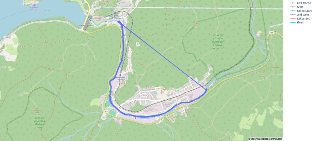
To get everyone up to speed briefly a GPX file is a standard type of file output by most consumer GPS receivers and sports watches. You can also download a GPX file of your STRAVA activities from the STRAVA website. This GPX file contains a list of timestamped positions that the ‘gpxsplits’ tool searches through. It interpolates between these positions checking for an intercept with a ‘virtual beam’ or ‘gate’ that the user can define using a JSON file. Then it logs all of these intercept times and from this calculates the elapsed time between gates and the subsequent split times. (More detailed instructions can be found in the README on the ‘gpxsplits’ github)

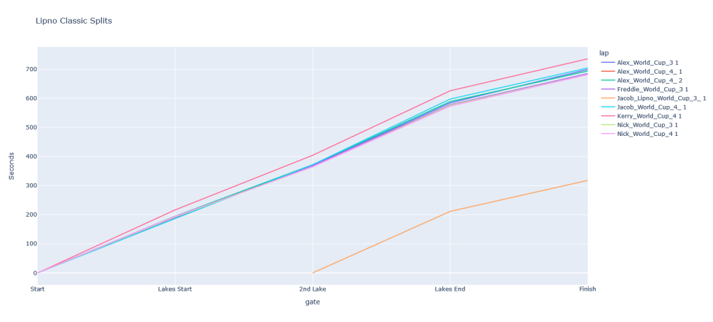
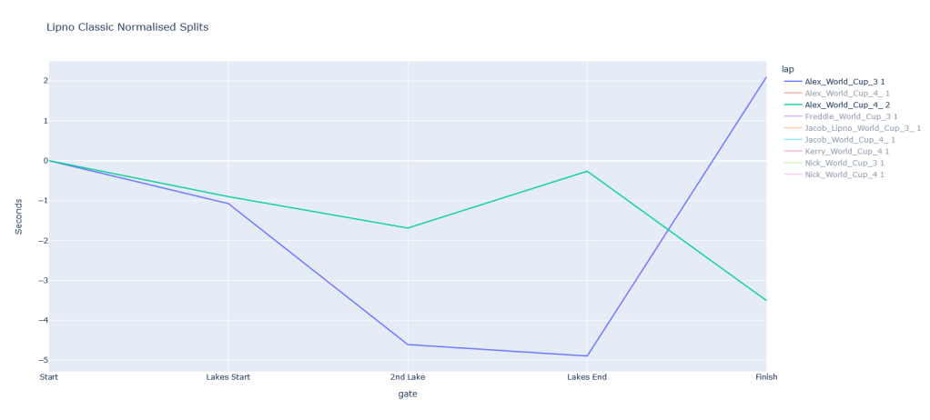
My favorite part about this though is the graphs. These graphs are very useful for visualizing the information and can reveal some interesting insights. The first graph, shown here is simple enough to interpret; simply showing the split time for each gate. However, by normalizing this to the average time, we can better compare each run (see below). Here zero on the y-axis represents the average time taken to complete a section and we then can see by how much each run was up or down on this time though the different sections. Thus a line with a positive gradient indicates the run in this section was slower than the average, while a run with a negative gradient shows a given section of a run was faster than the average.

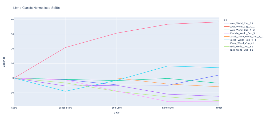
Looking at my two world cup races we can see they were both below the team average (yay me!) but to my surprise the white water sections at the start and end were much faster in my first run. However, on my second run it seems I really pulled my finger out over the lakes, allowing me to knock a few seconds off overall.

Meanwhile Alex’s traces tell a fun story. On both runs he managed a similar pace over the initial section of white water, but he tried much harder over the first lake in the first run. Unfortunately this led to a swim in the final section of white water. This meant he didn’t get an official time for this run, but we can see from his GPS watch that a lot of time was lost due to this regardless. On his second run he took the lakes at a more manageable pace leaving enough in the tank to handle the final rapid, securing a faster time overall.

This is all very fascinating but anyone knowledgeable on GPS or GNSS systems are probably asking how accurate these times are. This is quite a difficult question to answer, but it is largely dependent upon the accuracy of the sports watch being used. Sadly most manufacturers are fairly tight-lipped on this information and there is only limited information online about this. Furthermore what information there is, tends to only be concerned with the accuracy of the distance traveled and does not investigate the time component. Fortunately for us we can make a rough estimation of our accuracy by comparing the GPX split times to the official race time.

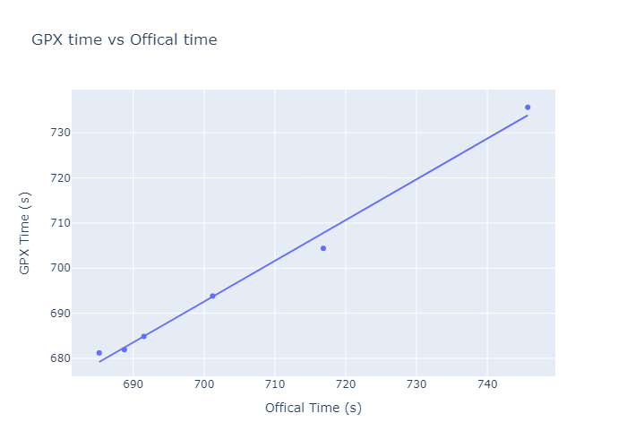
A quick visual analysis of the above plot confirms a good degree of correlation and importantly the finishing order of all the athletes (in the British team) has been preserved. When examining the numbers we see that the difference between GPX times and the official times has a standard deviation of 2.96s. This is reasonably high, however at least some of the error can be explained by the fact that the mean discrepancy between GPX and official times is -15.28s. This indicates I’ve done a relatively poor job of guesstimating where the start and finish beams were. Given the athletes were probably not traveling at a constant velocity across these 15 seconds, this gate error will have contributed to the standard deviation. Still given most basic GPS receivers are quoted to have a 95% error of around ~10m I am relatively impressed by the 2.96s error. This and the preservation of the finishing order gives me enough confidence that the ‘gpxtool’ can be used as a training aid, but I would hold off using it for official timing purposes.

It should be noted that this is a relatively brief investigation with only a few data points from the British team. If there are any other paddlers who could contribute their GPX files from either the Lipno World or Czech Cup races to improve this investigation that would be greatly appreciated. As would anyone who can give me better estimations for the start and finish beams.

In an ideal world I’d do a proper study where we survey in the beam locations, collect much larger data samples and potentially compare the sports watches to some more advanced techniques (RTK/PPP for you navigation nerds!), but for now this will have to do.

In the meantime I’m looking to develop this tool further. Two key features for improving useability are a UI tool for creating courses and a way to easily download GPX files from STRAVA or Garmin. UI stuff in particular is way outside my area of expertise, so if anyone out there fancies lending a hand please jump in. Everything is available open source on GitHub under an MIT license.

Happy Paddling!